使用Python画带空气阻力的抛体运动的轨迹

Projectile Motion with Air Resistance

Problem 2.9

Calculate the trajectory of your cannon shell including both air drag and the
Reduced air density at high altitudes so that you can reproduce the results in
Figure2.5.Perform your calculation for different firing angles and determine the
Value of the angle that gives the maximum range.

Solution with Python

同样由上一周Euler's Method的思路解决

Step.1 引入需要的作图包

import math
import numpy as np
from matplotlib import pyplot as plt

Step.2 定义函数与初值

由于需要考虑等温过程与绝热过程两个过程，跟丁峰同学讨论过后，我不太喜欢他把两个过程合并到一起的做法（尽管两个过程的函数基本相似），想了一下宁愿写丑一点，所以这里我把两个过程的$B$值分开做了计算（最后得出的图也跟丁峰有点点不一样）。

更具体的说明在代码上已经写了详尽的注释。

def PMotion(v,theta,T_0,select):
    v_x = v*math.cos(theta * math.pi/180);      #set initial speed constant in x 
    v_y = v*math.sin(theta * math.pi/180);      #set initial speed constant in y 
    a = 0.0065;                                 #set acceleration
    dt = 0.01;                                  #set time steps 
    y_0 = 10000.0;                              #initial sea height 
    alpha = 2.5;                                #set exponent alpha for air
    x = 0.0;                                    #initial position 
    y = 0.0;                                    #initial position 
    t = 0.0;                                    #set initial time 
    g = 9.8;                                    #set gravity acceleration
    B_0 = 0.00004;
    
    distance=[[]for i in range(3)];             #create a sequence to store x,y,t
    distance[0].append(x);
    distance[1].append(y);
    
    #select the model of approximation
    if select<0:                                #negative for isothermal approximation
        def rho(height):
            return math.exp(-height/y_0);       #(2.23)
        while y >= 0:
            B = B_0 * math.exp(-y/10000);
            a_x = -B * rho(y) * v * v_x;
            a_y = -g -B * rho(y) * v * v_y;
            x = x + v_x * dt;                   #Position in x as function of speed 
            y = y + v_y * dt;                   #Position in y as function of speed
            v_x = v_x + a_x * dt;               #Euler's solution in x 
            v_y = v_y + a_y * dt;               #Euler's solution in y 
            t = t + dt;                         #time steps
            v = math.sqrt(v_x * v_x + v_y * v_y);    #total speed
            distance[0].append(x/1000) 
            distance[1].append(y/1000)
        distance[2].append(t)
        return distance

    else:                                       #positive for adiabatic approximation
        def rho(height):
            return (1 - a*height/T_0)**alpha    #(2.24)
        while y >= 0:
            B = B_0 * math.pow((1-(6.5*0.001*y/300)),2.5);
            a_x = -B * rho(y) * v * v_x;
            a_y = -g -B * rho(y) * v * v_y;
            x = x + v_x * dt;                   #Position in x as function of speed 
            y = y + v_y * dt;                   #Position in y as function of speed
            v_x = v_x + a_x * dt;               #Euler's solution in x 
            v_y = v_y + a_y * dt;               #Euler's solution in y 
            t = t + dt;                         #time steps
            v = math.sqrt(v_x * v_x + v_y * v_y);    #total speed
            distance[0].append(x/1000) 
            distance[1].append(y/1000)
        distance[2].append(t)
        return distance

define结束后，给出函数的初值。

#set function parameter
velocity = 700.0;                     #set initial speed
T_0 = 300;

画图的部分。

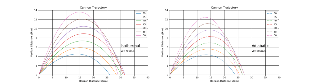
#plot the isothermal case
plt.subplot(1,2,1)
for i in range(7):
    angle= i * 5 + 30                  #set a series of theta
    d = PMotion(velocity,angle,T_0,-1) #-1 to select isothermal approximation
    plt.plot(d[0],d[1],linestyle='-',linewidth=1.0,label=angle)
    #print angle,d[0][-1],d[2][0]
plt.grid(True,color='k')
plt.title('Cannon Trajectory')
plt.text(30,6,'Isothermal',fontsize=15)
plt.text(30,5,'v0=700m/s')
plt.xlabel('Horizon Distance x(km)')
plt.ylabel('Vertical Distance y(km)')
plt.xlim(0,40)
plt.ylim(0,14)
plt.legend()

#plot the adiabatic case
plt.subplot(1,2,2)
for i in range(7):
    angle= i * 5 + 30                 #set a series of theta
    d = PMotion(velocity,angle,T_0,1) #1 to select adiabatic approximation
    plt.plot(d[0],d[1],linestyle='--',linewidth=1.0,label=angle)
    #print angle,d[0][-1],d[2][0]
plt.grid(True,color='k')
plt.title('Cannon Trajectory')
plt.text(30,6,'Adiabatic',fontsize=15)
plt.text(30,5,'v0=700m/s')
plt.xlabel('Horizon Distance x(km)')
plt.ylabel('Vertical Distance y(km)')
plt.xlim(0,40)
plt.ylim(0,14)
plt.legend()
plt.show()